Machine Learning - Linear Regression
Table of Content
- Logistic Regression
- Logistic Regression: Cost Function
- Computation Graph
- Logistic Regression Gradient descent
- Code Implementation
- Logic Regression in TensorFlow
Logistic Regression
Logistic regression is a learning algorithm used in a supervised learning problem when the output 𝑦 areall either zero or one. The goal of logistic regression is to minimize the error between its predictions andtraining data.
Example: Cat vs No - cat
Given an image represented by a feature vector 𝑥, the algorithm will evaluate the probability of a catbeing in that image.
\[Given \ x, \hat{y}=P(y=1|x), where \ 0 \leq \hat{y} \leq 1\]The parameters used in Logistic regression are:
-
The input features vector: \(x \in \mathbb{R}^{n_x}\) , where \(n_x\) is the number of features
for example the 64x64 RGB image, \(n_x = 64 \times 64 \times 3=12,288\) )
-
The trainig lable: \(y \in 0,1\)
-
\(m\) training example \(\{{(x^{(1)},y^{(1)}),(x^{(2)},y^{(2)}),…,(x^{(m)},y^{(m)})}\}\)
\[X={ \left[ \begin{array}{cccc} | & | & ... & |\\ x^{(1)} & x^{(2)} & ... & x^{(m)}\\ | & | & ... & | \end{array} \right ]}, X \in \mathbb{R}^{n_x \times m}, X.shape=(n_x, m)\] \[Y = [y^{(1)}, y^{(2)}, ...,y^{(m)}], Y \in \mathbb{R}^{1 \times m, Y.shape=(1,m)}\] -
The weights: \(w \in \mathbb{R}^{n_x}\) , where \(n_x\) is the number of features
-
The threshold: \(b \in \mathbb{R}\)
-
The output (sigmoid function): \(z = w^T x + b\) \(\hat{y} = a = \sigma(w^Tx+b)=\sigma(z)=\frac{1}{1+e^{-z}}\)
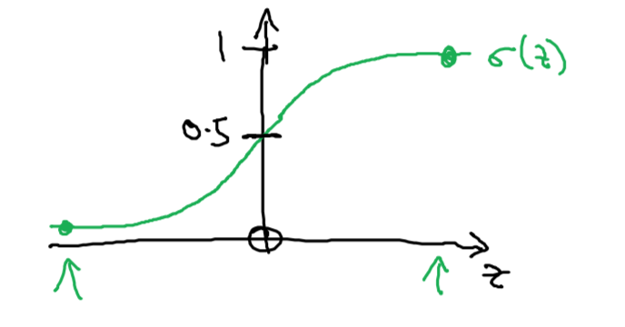
Some observations from the graph:
- If \(z\) is a large positive number, then \(\sigma(z)=1\)
- If \(z\) is small or large negative number, then \(\sigma(z)=0\)
- If \(z=0\) ,then \(\sigma(z)=0.5\)
Logistic Regression: Cost Function
To train the parameters \(w\) and \(b\) , we need to define a cost function.
Recap:
\[\hat{y} = a = \sigma(w^Tx+b)=\sigma(z)=\frac{1}{1+e^{-z}}\] \[Given \ \{{(x^{(1)},y^{(1)}),(x^{(2)},y^{(2)}),…,(x^{(m)},y^{(m)})}\}, want \ {{\hat{y}}^{(i)} \approx y^{(i)}}\]Loss (error) function
The loss function measures the discrepancy between the prediction \({\hat{y}}^{(i)}\) and the desired output \(y^{(i)}\) . In other words, the loss function computes the error for a single training example.
\[L({\hat{y}}^{(i)},y^{(i)})=\frac{1}{2}{({\hat{y}}^{(i)}-y^{(i)})}^2\]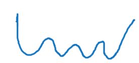
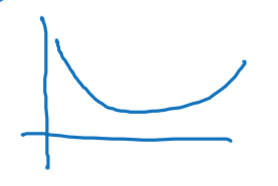
- If \(y^{(i)}=1\) : \(L({\hat{y}}^{(i)},y^{(i)})=-log({\hat{y}}^{(i)})\) where \(log({\hat{y}}^{(i)})\) and and \({\hat{y}}^{(i)}\) should be close to 1
- If \(y^{(i)}=0\) : \(L({\hat{y}}^{(i)},y^{(i)})=-log(1-{\hat{y}}^{(i)})\) where \(log(1-{\hat{y}}^{(i)})\) and \({\hat{y}}^{(i)}\) should be close to 0
Cost function
The cost function is the average of the loss function of the entire training set. We are going to find the parameters \(w\) and \(b\) that minimize the overall cost function.
\[J(w,b)=\frac{1}{m} \sum\limits_{i=1}^m L({\hat{y}}^{(i)},y^{(i)})=-\frac{1}{m}\sum\limits_{i=1}^m [y^{(i)}log({\hat{y}}^{(i)})+(1-y^{(i)})log(1-{\hat{y}}^{(i)})]\]Gradient Descent Recap:
\(\hat{y} = a = \sigma(w^Tx+b)=\sigma(z)=\frac{1}{1+e^{-z}}\) \(J(w,b)=\frac{1}{m} \sum\limits_{i=1}^m L({\hat{y}}^{(i)},y^{(i)})=-\frac{1}{m}\sum\limits_{i=1}^m [y^{(i)}log({\hat{y}}^{(i)})+(1-y^{(i)})log(1-{\hat{y}}^{(i)})]\)
Want to find \(w,b\) that minimize \(J(w,b)\)
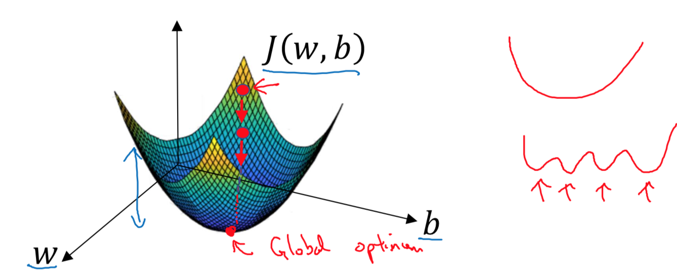
Every iteration will update \(w\) and \(b\) as following, the \(\alpha\) is the “learing rate”
\[w:=w - \alpha \frac{\mathrm{d}J(w,b)}{\mathrm{d}w}\] \[b:=b - \alpha \frac{\mathrm{d}J(w,b)}{\mathrm{d}b}\]And in code, the derivative \(\frac{\mathrm{d}J(w,b)}{\mathrm{d}w}\) is the variable of “dw” and derivative \(\frac{\mathrm{d}J(w,b)}{\mathrm{d}b}\) is the variable of “db”
\[w := w - \alpha \mathrm{d}w\] \[b := b - \alpha \mathrm{d}b\]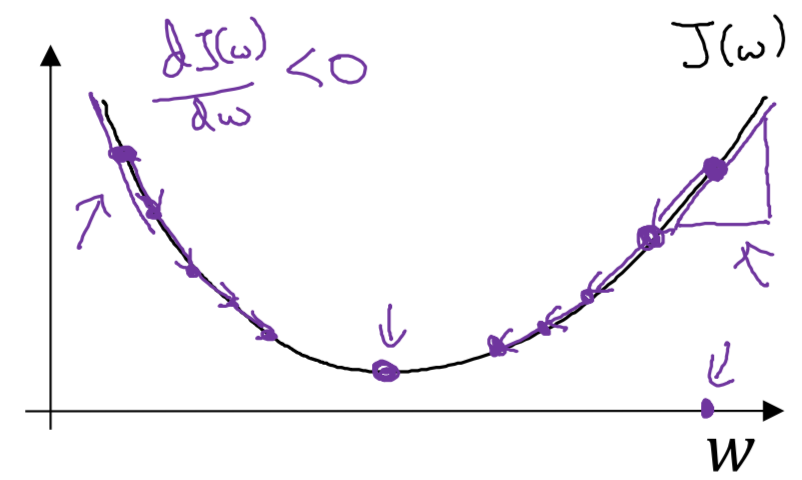
Computation Graph
Computation Graph

Derivatives with a Computation Graph

Logistic Regression Gradient descent
\[z = w^T x + b\] \[\hat{y} = a = \sigma(w^Tx+b)=\sigma(z)=\frac{1}{1+e^{-z}}\] \[L({\hat{y}}^{(i)},y^{(i)})=-(y^{(i)}log({\hat{y}}^{(i)})+(1-y^{(i)})log(1-{\hat{y}}^{(i)}))\] \[J(w,b)=\frac{1}{m} \sum\limits_{i=1}^m L({\hat{y}}^{(i)},y^{(i)})=-\frac{1}{m}\sum\limits_{i=1}^m [y^{(i)}log({\hat{y}}^{(i)})+(1-y^{(i)})log(1-{\hat{y}}^{(i)})]\]Logistic regression derivatives
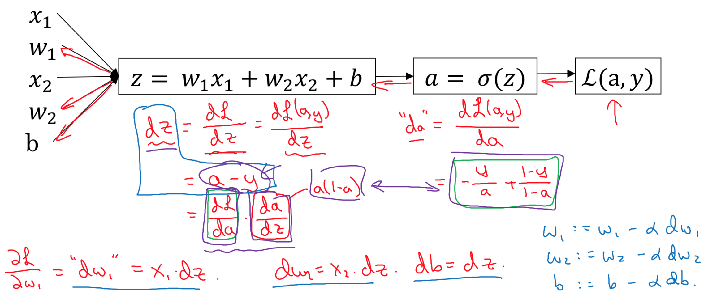
\(dz = (a-y)\) \(dw_1 = x_1*dz\) \(dw_2=x_2*dz\) \(db = dz\)
Vectorization
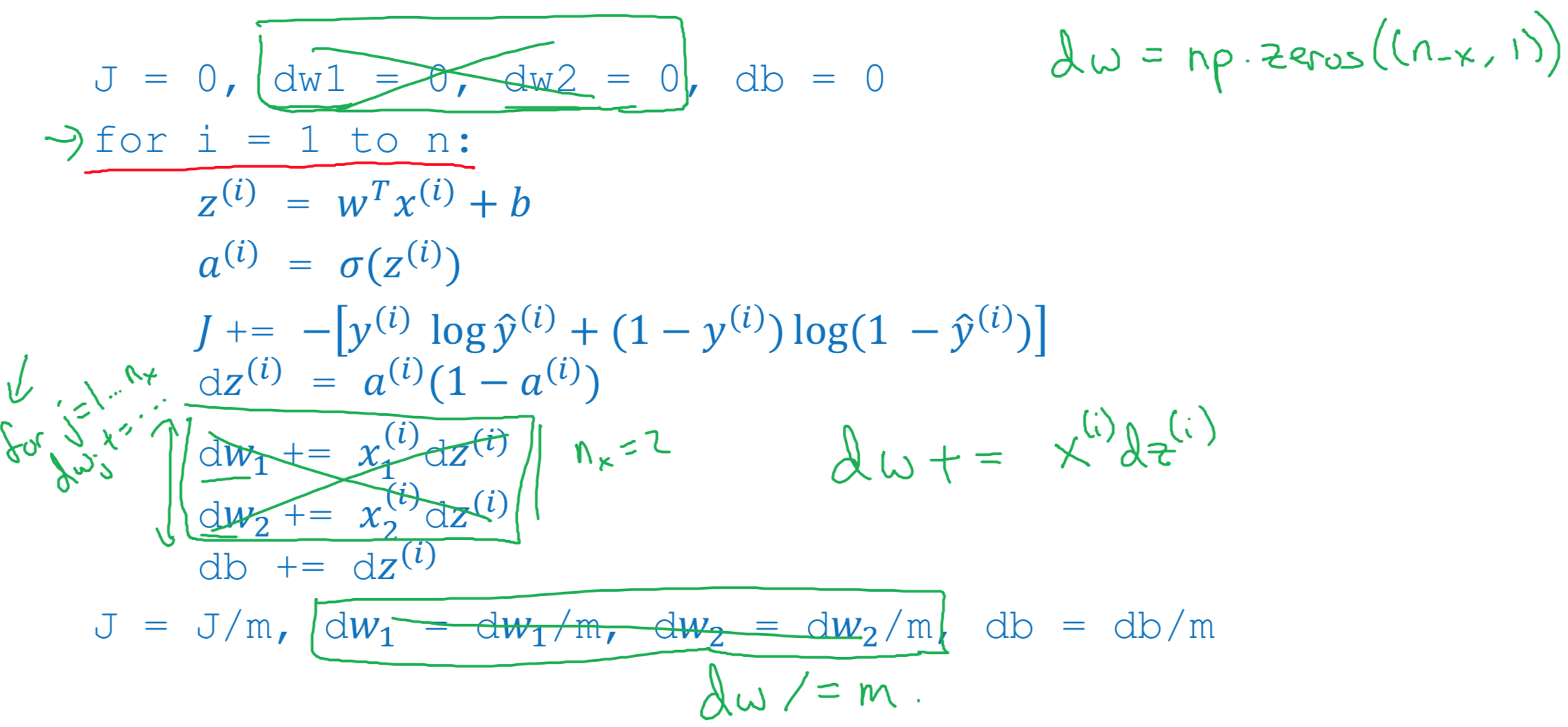
Vectorizing Logistic Regression
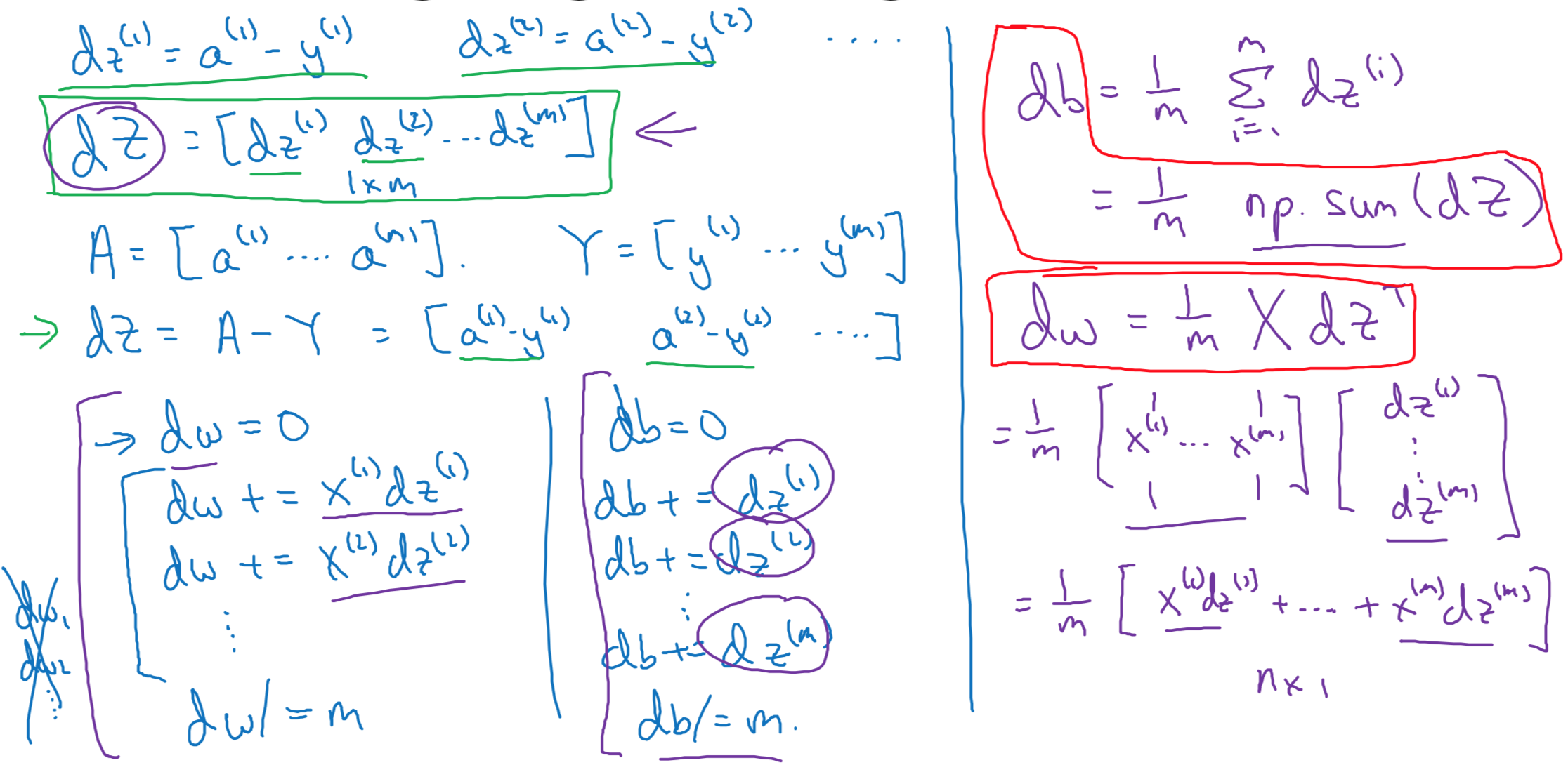
\(dZ = A-Y\) \(dB = \frac{1}{m} np.sum(dZ)=\frac{1}{m} \sum\limits_{i=1}^m (a^{(i)}-y^{(i)})\) \(dW=\frac{1}{m} XdZ^T=\frac{1}{m}X(A-Y)^T\)
Implementing Logistic Regression

Code Implementation
1
2
3
4
5
6
7
8
9
10
11
12
13
14
15
16
17
18
19
20
21
22
23
24
25
26
27
28
29
30
31
32
33
34
35
36
37
38
39
40
41
42
43
44
45
46
47
48
49
50
51
52
53
54
55
56
57
58
59
60
61
62
63
64
65
66
67
68
69
70
71
72
73
74
75
76
77
78
79
80
81
82
83
84
85
86
87
88
89
90
91
92
93
94
95
96
97
98
99
100
101
102
103
104
105
106
107
108
109
110
111
112
113
114
115
116
117
118
119
120
121
122
123
124
125
126
127
128
129
130
131
132
133
134
135
136
137
138
139
140
141
142
143
144
145
146
147
148
149
150
151
152
153
154
155
156
157
158
159
160
161
162
163
164
165
166
167
168
169
170
171
import numpy as np
import matplotlib.pyplot as plt
import h5py
import scipy
from PIL import Image
from scipy import ndimage
from lr_utils import load_dataset

%matplotlib inline

# Loading the data (cat/non-cat)
# train_set_x_orig.shape = (209, 64, 64, 3)
# train_set_y.shape = (1, 209)
# test_set_x_orig.shape = (50, 64, 64, 3)
# test_set_y.shape = (1, 50)
train_set_x_orig, train_set_y, test_set_x_orig, test_set_y, classes = load_dataset()

# Number of training examples: m_train = 209
# Number of testing examples: m_test = 50
# Height/Width of each image: num_px = 64
m_train = train_set_y.shape[1]
m_test = test_set_y.shape[1]
num_px = train_set_x_orig.shape[1]

# train_set_x_flatten shape: (12288, 209)
# test_set_x_flatten shape: (12288, 50)
train_set_x_flatten = train_set_x_orig.reshape(train_set_x_orig.shape[0], -1).T
test_set_x_flatten = test_set_x_orig.reshape(test_set_x_orig.shape[0], -1).T

# standardize our dataset.
train_set_x = train_set_x_flatten / 255.
test_set_x = test_set_x_flatten / 255.

# GRADED FUNCTION: sigmoid
def sigmoid(z):
    s = 1 / (1 + np.exp(-z))
    return s

# GRADED FUNCTION: initialize_with_zeros
def initialize_with_zeros(dim):
    w = np.zeros(shape=(dim, 1))
    b = 0
    assert(w.shape == (dim, 1))
    assert(isinstance(b, float) or isinstance(b, int))
    return w, b

# GRADED FUNCTION: propagate
def propagate(w, b, X, Y):
    m = X.shape[1]

    # FORWARD PROPAGATION (FROM X TO COST)
    A = sigmoid(np.dot(w.T, X) + b)  # compute activation
    cost = (- 1 / m) * np.sum(Y * np.log(A) + (1 - Y) * (np.log(1 - A)))  # compute cost

    # BACKWARD PROPAGATION (TO FIND GRAD)
    dw = (1 / m) * np.dot(X, (A - Y).T)
    db = (1 / m) * np.sum(A - Y)

    assert(dw.shape == w.shape)
    assert(db.dtype == float)
    cost = np.squeeze(cost)
    assert(cost.shape == ())

    grads = {"dw": dw,
             "db": db}

    return grads, cost

# GRADED FUNCTION: optimize

def optimize(w, b, X, Y, num_iterations, learning_rate, print_cost = False):
    costs = []

    for i in range(num_iterations):

        # Cost and gradient calculation (≈ 1-4 lines of code)
        grads, cost = propagate(w, b, X, Y)

        # Retrieve derivatives from grads
        dw = grads["dw"]
        db = grads["db"]

        # update rule (≈ 2 lines of code)
        w = w - learning_rate * dw  # need to broadcast
        b = b - learning_rate * db

        # Record the costs
        if i % 100 == 0:
            costs.append(cost)

        # Print the cost every 100 training examples
        if print_cost and i % 100 == 0:
            print ("Cost after iteration %i: %f" % (i, cost))

    params = {"w": w,
              "b": b}

    grads = {"dw": dw,
             "db": db}

    return params, grads, costs

# GRADED FUNCTION: predict

def predict(w, b, X):

    m = X.shape[1]
    Y_prediction = np.zeros((1, m))
    w = w.reshape(X.shape[0], 1)

    # Compute vector "A" predicting the probabilities of a cat being present in the picture
    A = sigmoid(np.dot(w.T, X) + b)

    for i in range(A.shape[1]):
        # Convert probabilities a[0,i] to actual predictions p[0,i]
        Y_prediction[0, i] = 1 if A[0, i] > 0.5 else 0

    assert(Y_prediction.shape == (1, m))

    return Y_prediction

# GRADED FUNCTION: model
def model(X_train, Y_train, X_test, Y_test, num_iterations=2000, learning_rate=0.5, print_cost=False):

    # initialize parameters with zeros (≈ 1 line of code)
    w, b = initialize_with_zeros(X_train.shape[0])

    # Gradient descent (≈ 1 line of code)
    parameters, grads, costs = optimize(w, b, X_train, Y_train, num_iterations, learning_rate, print_cost)

    # Retrieve parameters w and b from dictionary "parameters"
    w = parameters["w"]
    b = parameters["b"]

    # Predict test/train set examples (≈ 2 lines of code)
    Y_prediction_test = predict(w, b, X_test)
    Y_prediction_train = predict(w, b, X_train)

    # Print train/test Errors
    print("train accuracy: {} %".format(100 - np.mean(np.abs(Y_prediction_train - Y_train)) * 100))
    print("test accuracy: {} %".format(100 - np.mean(np.abs(Y_prediction_test - Y_test)) * 100))


    d = {"costs": costs,
         "Y_prediction_test": Y_prediction_test,
         "Y_prediction_train" : Y_prediction_train,
         "w" : w,
         "b" : b,
         "learning_rate" : learning_rate,
         "num_iterations": num_iterations}

    return d

# Plot learning curve (with costs)
learning_rates = [0.01, 0.001, 0.0001]
models = {}
for i in learning_rates:
    print ("learning rate is: " + str(i))
    models[str(i)] = model(train_set_x, train_set_y, test_set_x, test_set_y, num_iterations = 1500, learning_rate = i, print_cost = False)
    print ('\n' + "-------------------------------------------------------" + '\n')

for i in learning_rates:
    plt.plot(np.squeeze(models[str(i)]["costs"]), label= str(models[str(i)]["learning_rate"]))

plt.ylabel('cost')
plt.xlabel('iterations')

legend = plt.legend(loc='upper center', shadow=True)
frame = legend.get_frame()
frame.set_facecolor('0.90')
plt.show()
Logic Regression in TensorFlow
TBD